Unfolded neural network for deblur and denoise

Introduction

This project aims to deblur and denoise images, with a focus on the MNIST dataset. The methodology is based on the “Unfolded Forward Backward” approach, developed as part of my master’s thesis project at ENS Lyon. The code to produce the results of this blog post is available on my github account. I introduced in an other post blog unfolded neural network with the first model introduced in the article Learning Fast Approximations of Sparse Nonlinear Regression

Data

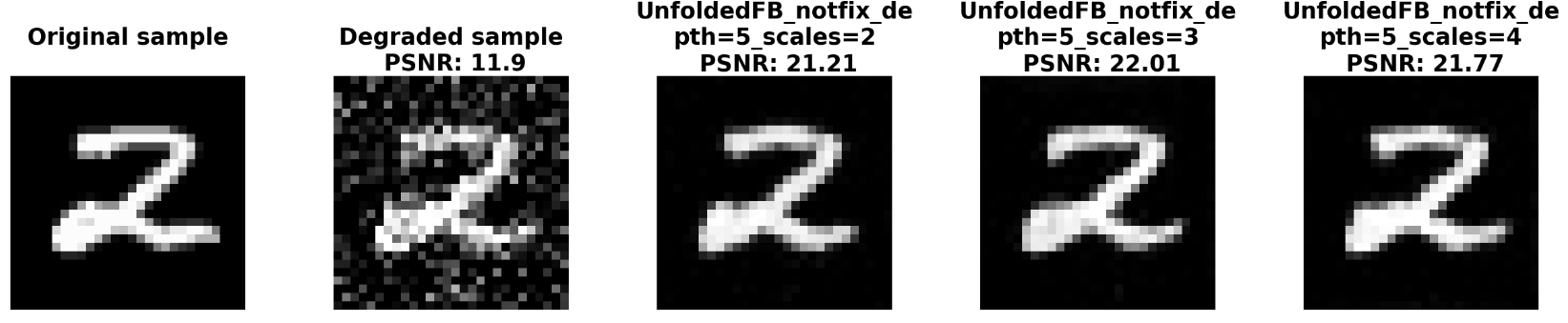
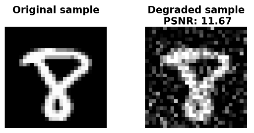
I worked with the standard MNIST dataset imported from the Keras library, consisting of 70,000 images, each of size \(28 \times 28\) pixels. To normalize these images, I divided each pixel’s value by 255 to bring them into the range of 0 to 1. To degrade the quality of the handwritten digits, I applied a Gaussian blur with a kernel size of \(7 \times 7\) and a standard deviation of 0.5. Subsequently, I introduced Gaussian noise with a standard deviation of 0.25, resulting in pairs of original and degraded images, as displayed below. We measured the difference between the degraded and original images using the traditional PSNR metric.

The main objective of this project is to create an estimator for the original image based on the degraded image. The quality of this estimator is assessed using the PSNR metric.

Model

\(\bullet\) I adopted the classical formalism of inverse problems:
The goal of solving an \(\textit{inverse problem}\) is to create an estimator, denoted as \(\boldsymbol{\widehat{x}} \in \mathbb{R}^{28^2}\), from a set of observed measurements, represented as the degraded images \(\boldsymbol{y} \in \mathbb{R}^{28^2}\). The objective is to create an estimator that is close to the ground truth data, the original image \(\boldsymbol{\bar{x}}\). In our case, we have \(\boldsymbol{y} = A\boldsymbol{\bar{x}} + \mathbf{\epsilon}, \text{ with } A \in \mathbb{R}^{28^2 \times 28^2} \text{ and } \mathbf{\epsilon} \sim \mathbb{N}(\mathbf{0}, \mathbf{\sigma^2 I})\). With \(A\) the gaussian blur and \(\mathbf{\epsilon}\) the gaussian noise.

\(\bullet\) The estimator \(\boldsymbol{\widehat{x}}\) for \(\boldsymbol{\bar{x}}\) is typically obtained by solving a variational problem, defined as follows: \(\begin{align} \widehat{\boldsymbol{x}} \in \underset{\boldsymbol{x} \in \mathbb{R}^{28^2}}{\arg \min}\left[\frac{1}{2}||\boldsymbol{y}-A\boldsymbol{x}||_2^2+\mathcal{P}(\boldsymbol{x})\right] \end{align}\) Here, \(||\boldsymbol{y}-A\boldsymbol{x}||_2^2\) represents the data fidelity term, ensuring that the degraded solution \(A\boldsymbol{\widehat{x}}\) is close to the degraded signal \(\boldsymbol{y}\). Additionally, \(\mathcal{P}: \mathbb{R}^{28^2} \rightarrow \mathbb{R}\) is a prior term. For more details on variational problems, you can refer to my Master’s thesis.

\(\bullet\) Choosing an appropriate prior term can be challenging. However, once a suitable prior term is chosen, it is possible to find the minimizer of equation (1) using proximal iterative methods like Forward-Backward:
Forward-Backward algorithm:
Assumption: \(\zeta := |||A^*A|||_2<2,\)
Input: \(\boldsymbol{y}\in \mathbb{R}^{28^2}\), step size \(\tau\in ]0,2\zeta^{-1}[,\)
\(x^0 = A^*y,\)
For \(n = 0, 1, 2, \ldots\):
\(\quad \quad \tilde{x}^{n}=x^n-\tau A^*(Ax^n - \boldsymbol{y})\);
\(\quad \quad x^{n+1} = \operatorname{prox}_{\tau \mathcal{R}}(\tilde{x}^{n})\);
Output: \(\lim\limits_{n\rightarrow\infty}{x^n} \in{\arg\min\limits_{x \in \mathbb{R}^{28^2}}}\left[\dfrac{1}{2}||\boldsymbol{y}-A\boldsymbol{x}||_2^2+\mathcal{P}(\boldsymbol{x})\right]\)

• Remark: Let \(h: \mathcal{H} \rightarrow \mathbb{R},\) \(\forall x \in \mathcal{H} \quad \operatorname{prox}_{\tau h}(x)=\underset{y \in \mathcal{H}}{\operatorname{argmin}} \frac{1}{2 \tau}\|x-y\|^{2}+h(y)\)

\(\bullet\) To address the challenge of selecting a suitable prior term, the iterations of Forward-Backward can be unfolded to learn the prior through deep-learning frameworks. The first unfolded network was introduced in the paper Learning Fast Approximations of Sparse Coding in 2010. To parameterize the unfolded network, I replaced the proximal operator of the prior with UNets, denoted as \(U_{\theta^k}\). To facilitate the learning process, I limited the number of iterations to 5. The algorithm is defined as follows:\(\\\)

Unfolded Forward-Backward architecture network:
Assumption: \(\zeta:=|||A^*A|||_2 < 2,\, {U_{\theta^k}}_{k\in[0;4]},\) UNets,
Input: \(\boldsymbol{y}\in \mathbb{R}^{28^2}\), step size \(\tau \in ]0,2\zeta^{-1}[,\)
\(x^0 = A^*y,\)
For \(n = 0, 1, 2, \ldots 4\):
\(\quad \quad \tilde{x}^{n}=x^n- \tau A^*(y - Ax^n);\)
\(\quad \quad x^{n+1} = U_{\theta^{n+1}}(\tilde{x}^{n})\);
Output: \(f_\theta(y)=x^5\)

\(\bullet\) I trained the unfolded network using \(300\) of the \(70\,000\) images from the MNIST dataset. I reserved \(10\,000\) images for testing. It is possible to play with the number of iterations, which corresponds to the layers of our neural network, and the number of scales of the UNets, which determine the size of the UNets. I kept the number of layers fixed at 5 and the number of scales within the set \(\{2, 3, 4\}\).

Results

\(\bullet\) I minimized the cost function, which is defined as the mean squared error on the \(300\) training images: \(\sum\limits_{i \in [1,300]} \|\bar{x}_i - f_\theta(y)\|^2_2\).

\(\bullet\) In the following plot, the training was performed for 50 epochs using the Adam algorithm. The red curve represents the PSNR calculated on the test set, and the blue curve represents the value of the loss function with respect to the number of epochs. Additionally, a table displaying the mean PSNR on the test set, the number of parameters, and the training time is provided.

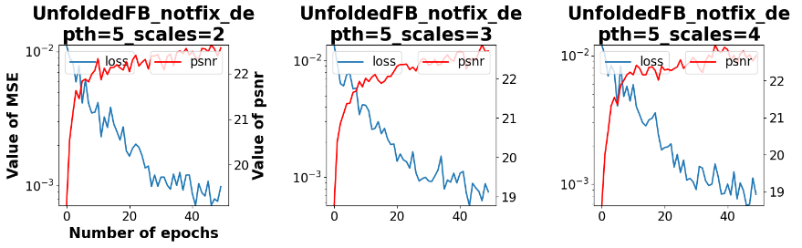
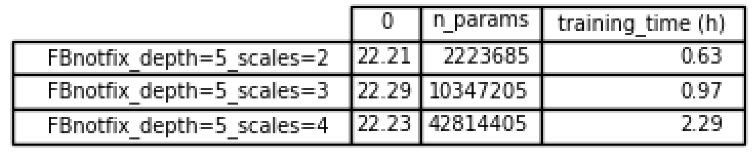
\(\bullet\) It is evident that there is no significant difference between the three settings. This can be attributed to the relatively low number of training epochs. In my thesis, it was observed that a higher number of parameters leads to better PSNR results. However, training for hundreds of epochs on my personal computer, which lacks a GPU, is time-consuming. Additionally, it’s noteworthy that the training time increases with a higher number of scales.
Here is an example of a reconstructed sample, demonstrating the quality of the results: