Edouard Chappon

Introduction

The objective is to implement the first unfolded Neural Network (NN) described in Learning Fast Approximations of Sparse Nonlinear Regression. I also implement 3 variants of it introduced in Theoretical Linear Convergence of Unfolded ISTA and its Practical Weights and Thresholds which gives the proof of 3 theorems we will explain and empiricaly verify.
The code used for this project is available on GitHub. I used other unroled network to learn how to deblur and denoise images from mnist daset in an other post blog .

Sparse signal recovery and Data

In this blog post we will solve an sparse signal recovery problem. We aim to recover a sparse vector $x^* \in \mathbb{R}^n$ from its noisy linear measurments $y \in \mathbb{R}^m$, with $m=250$ and $n=500$: $y=Ax^*+\epsilon$ Where $\epsilon \in \mathbb{R}^m$ an additive Gaussian white noise to have a Signal to Noise Rate (SNR) of $30dB$, and $A \in \mathbb{R}^{m\times n}$ with each entries sampled as Gaussian distribution $A_{i,j}∼\mathcal{N}(0,1/m)$ and then we normalize the columns.
We define $x^*$ as a Gaussian vector of $\mathbb{R}^n$ where we set each entry to $0$ with a probability of $p_b=0.1$ to make it sparse. $1\,000$ such data are generated for the train set and $1\,000$ others for the test set.

Iterative Shrinkage Thresholding Algorithm (ISTA)

In inverse problem, the estimator $\widehat{x}$ of $x^*$ is classically obtained by the minimization of the sum of a datafidelity term $||y-Ax||_2^2$ and the regularization $\lambda \|x\|_1$ to enforce the sparsity of the solution. This problem is known as LASSO problem:
$\begin{align} \widehat{x} \in \underset{x \in \mathbb{R}^{n}}{\arg\min}\left[\dfrac{1}{2}||y-Ax||_2^2+ \lambda \|x\|_1 \right] \end{align}$

ISTA is an iterative algorithm which aims to solve $(1)$, it converges sublinearly (see the link for more explanations of that algorithm):

ISTA:
Assumption: $\zeta := |||A^*A|||_2<2,$
Input: $y\in \mathbb{R}^{m}$, step size $\tau\in ]0,2\zeta^{-1}[,$
$x^0 = A^*y,$
For $k = 0, 1, 2, \ldots$:
$\quad \quad \tilde{x}^{k}=x^n-\tau A^*(Ax^k - y)$
$\quad \quad x^{k+1} = \mathcal{S}_{\lambda/L}(\tilde{x}^{k}) \quad \quad \text{with} \; \;(\mathcal{S}_{\theta}(x))_i = \operatorname{sgn}(x_i)\operatorname{max}(|x_i|-\theta,0)$
Output: $\lim\limits_{k\rightarrow\infty}{x^k} \in{\arg\min\limits_{x \in \mathbb{R}^{n}}}\left[\dfrac{1}{2}||y-Ax||_2^2+\lambda||x||_1\right]$

Remark: $\mathcal{S}_\theta$ is called the soft thresholding function. It is a non-linear function.

Original LISTA

A neural network $d_\theta$ with $K$ layers and parametrized by $\theta$ is defined as:

\[\begin{align} d_\theta(y) = \eta^{K}\left(W^{K}_2 \dots \eta^{1}\left(W^{1}_2y + W^{1}_1\right) \dots + W^{K}_1\right) \quad\quad \text{with} \quad \theta = \{W^{1}_2, \ldots, W^{K}_2, W^{1}_1, \ldots, W^{K}_1\} \end{align}\]

The article Learning Fast Approximations of Sparse Nonlinear Regression introduce the first unrolled neural network called Learned ISTA (LISTA) by hilighting the fact that an iteration of ISTA looks like a layer of a neural network if we rearange iterations of ISTA as below and we assimilate $\mathcal{S}_{\theta^k}$ as the activation function:

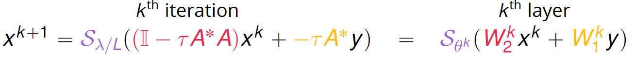
We fix number of layers $K=16$ and $x^0=\vec{0}$ LISTA network is defined as :

\[\begin{align} d_\theta^K(y) = S_{\theta^K}\left(W^{K}_2 \dots S_{\theta^1}\left(W^{1}_2x^0 + W^{1}_1y\right) \dots + W^{K}_1y\right) \quad \quad \text{with} \quad \theta = \{W^{1}_2, \ldots, W^{K}_2, \theta^1, \ldots, \theta^K, W^{1}_1, \ldots, W^{K}_1\} \end{align}\]

Remarks: Advantage of LISTA compare to ISTA is that when the parameters $\theta$ is trained it is cheap $\quad \quad\quad \;$ to evaluate. ISTA requires thousands of iterations where LISTA requires only few tens. $\quad \quad\quad \;$ This network and ones we will see further have been trained with Adam for $2\,500$ epochs. $\quad \quad\quad \;$ With thoses settings, LISTA has $6\,000\,016$ parameters to train.

To start with a good initialization and make training easier, we start training with :

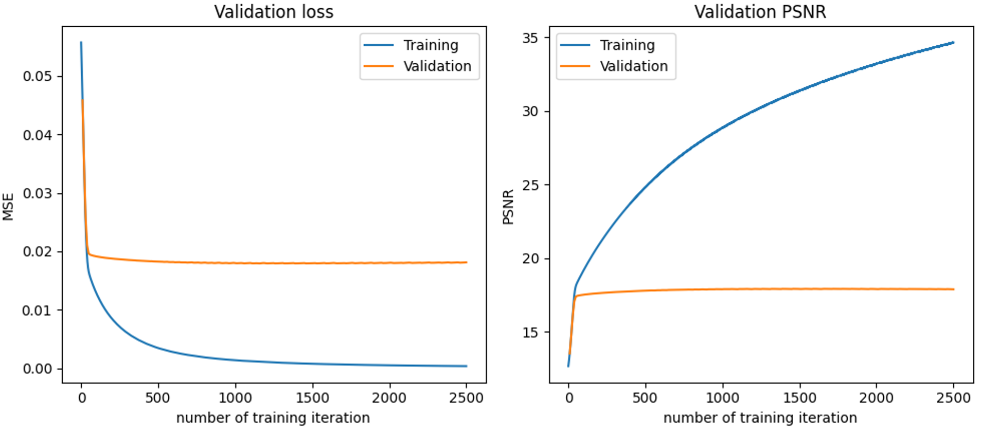
$$\begin{align*} \forall k \in [1,\ldots, K], \quad&\theta^k = \lambda/L \\ & W_2^k = (\mathbb{I}-\tau A^*A) \quad \quad \text{with} \quad \tau=L^{-1}\\ & W_1^k = -\tau A^* \end{align*}$$

Here are the curves of loss and PSNR of the traini and validation/test sets (which contains $1\,000$ data each) during the training phase. The next parts explains and illustrates theoriticals results of convergence for LISTA networks and 3 variations.

Necessary condition for LISTA convergence

Theorems are prooved in the paper Theoretical Linear Convergence of Unfolded ISTA and its Practical Weights and Thresholds.

$\textbf{Assumption 1:}$ The signal $x^{*}$ and the observation noise $\epsilon$ are sampled from the following set:

\[\left(x^{*}, \varepsilon\right) \in \mathcal{X}(B, s, \sigma) \triangleq\left\{\left(x^{*}, \varepsilon\right)|| x_{i}^{*} \mid \leq B, \forall i,\left\|x^{*}\right\|_{0} \leq s,\|\varepsilon\|_{1} \leq \sigma\right\} .\]

$\textbf{Theorem 1:}$ Given $\theta=\left\{W_{1}^{k}, W_{2}^{k}, \theta^{k}\right\}_{k=0}^{\infty}$ and $x^{0}=0$, let $y$ be observed by (1) and $\left\{d^k_\theta\right\}_{k=1}^{\infty}$ be generated layer-wise by LISTA (3). If the following holds uniformly for any $\left(x^{*}, \epsilon\right) \in \mathcal{X}(B, s, 0)$:

\[d^k_\theta(y) \rightarrow x^{*}, \quad \text { as } k \rightarrow \infty\]

and $\left\{W_{2}^{k}\right\}_{k=1}^{\infty}$ are bounded:

\[\left\|W_{2}^{k}\right\|_{2} \leq B_{W}, \quad \forall k=0,1,2, \cdots\]

then $\theta=\left\{W_{1}^{k}, W_{2}^{k}, \theta^{k}\right\}_{k=0}^{\infty}$ must satisfy:

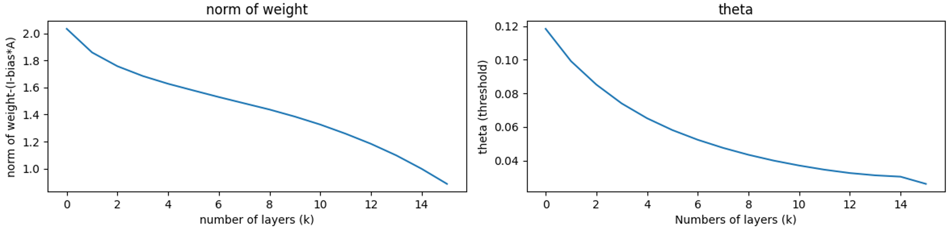
\[\begin{aligned} & W_{2}^{k}-\left(\mathbb{I}-W_{1}^{k} A\right) \rightarrow 0, \quad \text { as } k \rightarrow \infty \\ & \theta^{k} \rightarrow 0, \quad \text { as } k \rightarrow \infty \end{aligned}\]

$\textbf{explanation:}$ This theorem means that under mild assumption, and not noised data, LISTA network verify that thresholds $\theta^k \rightarrow 0$ and we have the weight coupling $\left(\mathbb{I}-W_{1}^{k} A\right) \rightarrow W_{2}^{k}$ which is verified for ISTA. Next section introduce a variant of LISTA that leverages on this coupling.

Our results for weight coupling is not convincing because of the difference in the training method (cf the paper).

LISTA-CP and sufficient condition for convergence

Theorem 1 shows that we have a assymptotical weight coupling : $\left(\mathbb{I}-W_{1}^{k} A\right) \rightarrow W_{2}^{k}$. The idea of LISTA Partial weight Coupling (LISTA-CP) is to make this asymptotical equality true for all layers. Then we replace $W_1^k$ by $W^k$ and $W_2^k$ by $\left(\mathbb{I}-W^{k} A\right)$ which gives the NN:

\[\begin{align} d_\theta^K(y) = S_{\theta^K}\left(\left(\mathbb{I}-W^{K} A\right) \dots S_{\theta^1}\left(\left(\mathbb{I}-W^{1} A\right)x^0 + W^{1}y\right) \dots + W^{K}y\right) \quad \quad \text{with} \quad \theta = \{W^{1}, \ldots, W^{K}, \theta^1, \ldots, \theta^K\} \end{align}\]

$\textbf{Theorem 2:}$ Given $\left\{W^{k}, \theta^{k}\right\}_{k=0}^{\infty}$ and $x^{0}=0$, let $\left\{x^{k}\right\}_{k=1}^{\infty}$ be generated by (4). If Assumption 1 holds and $s$ is sufficiently small, then there exists a sequence of parameters $\theta=\left\{W^{k}, \theta^{k}\right\}$ such that, for all $\left(x^{*}, \varepsilon\right) \in \mathcal{X}(B, s, \sigma)$, we have the error bound:

\[\begin{align} \left\|d^k_\theta(y)-x^{*}\right\|_{2} \leq s B \exp (-c k)+C \sigma, \quad \forall k=1,2, \cdots \end{align}\]

where $c>0, C>0$ are constants that depend only on $A$ and $s$.

$\textbf{explanation:}$ This theorem means that there exists, under mild assumptions, parameters $\theta$ such that our LISTA-CP network error estimation is bounded by a proportion of the noise level. That means that in the noiseless case, our network converge linearly to the signals in our training set. This is a better rate of convergence than ISTA which converges sublinearly.

$\textbf{Discussion:}$ The bound (5) clarifies the accelerated convergence of LISTA compared to ISTA. ISTA achieves a linear rate with a sufficiently large $\lambda$:

\[\begin{aligned} x^{k} \rightarrow \bar{x}(\lambda) \text{ sublinearly, } & \left\|\bar{x}(\lambda)-x^{*}\right\|=O(\lambda), & \lambda>0 \\ x^{k} \rightarrow \bar{x}(\lambda) \text{ linearly, } & \left\|\bar{x}(\lambda)-x^{*}\right\|=O(\lambda), & \lambda \text{ large enough. } \end{aligned}\]

The choice of $\lambda$ in LASSO introduces an inherent trade-off between convergence rate and approximation accuracy in solving the inverse problem. A larger $\lambda$ leads to faster convergence but a less accurate solution, and vice versa.

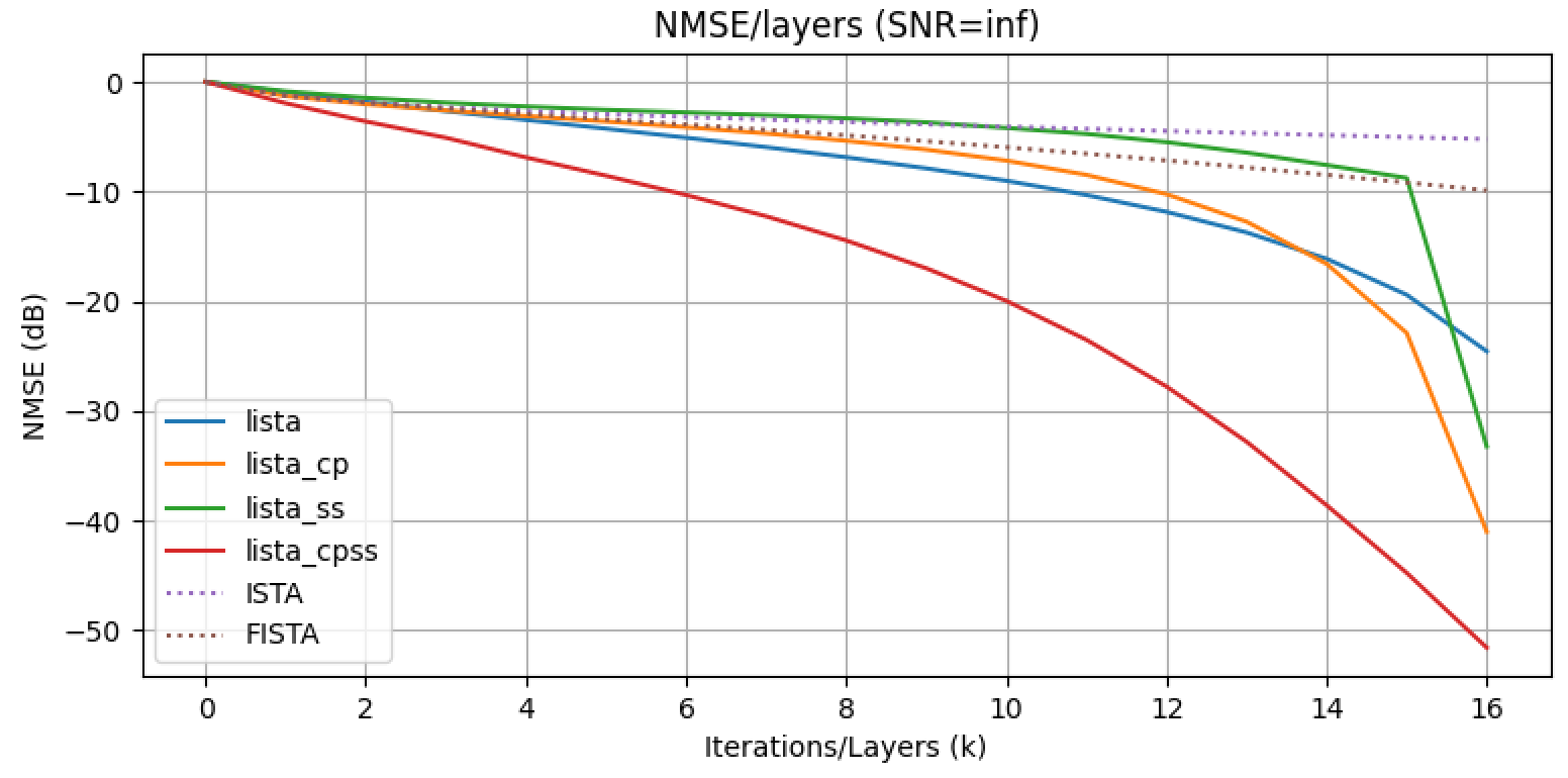
However, if $\lambda$ varies adaptively across iterations, a promising trade-off emerges. LISTA and LISTA-CP adopt this approach by training free thresholds $\{\theta^{k}\}_{k=1}^{K}$. LISTA and LISTA-CP learning-based algorithms achieve accurate solutions at a fast convergence rate. Theoretical results in Theorem 2 establish the existence of such a sequence $\{W^{k}, \theta^{k}\}_{k}$ in LISTA-CP. The following experimental results demonstrate empiricaly this convergence improvement. The recovery performance is evaluated by NMSE (in $\mathrm{dB}$ ):

\[\operatorname{NMSE}\left(\hat{x}, x^{*}\right)=10 \log _{10}\left(\frac{\mathbb{E}\left\|\hat{x}-x^{*}\right\|^{2}}{\mathbb{E}\left\|x^{*}\right\|^{2}}\right)\]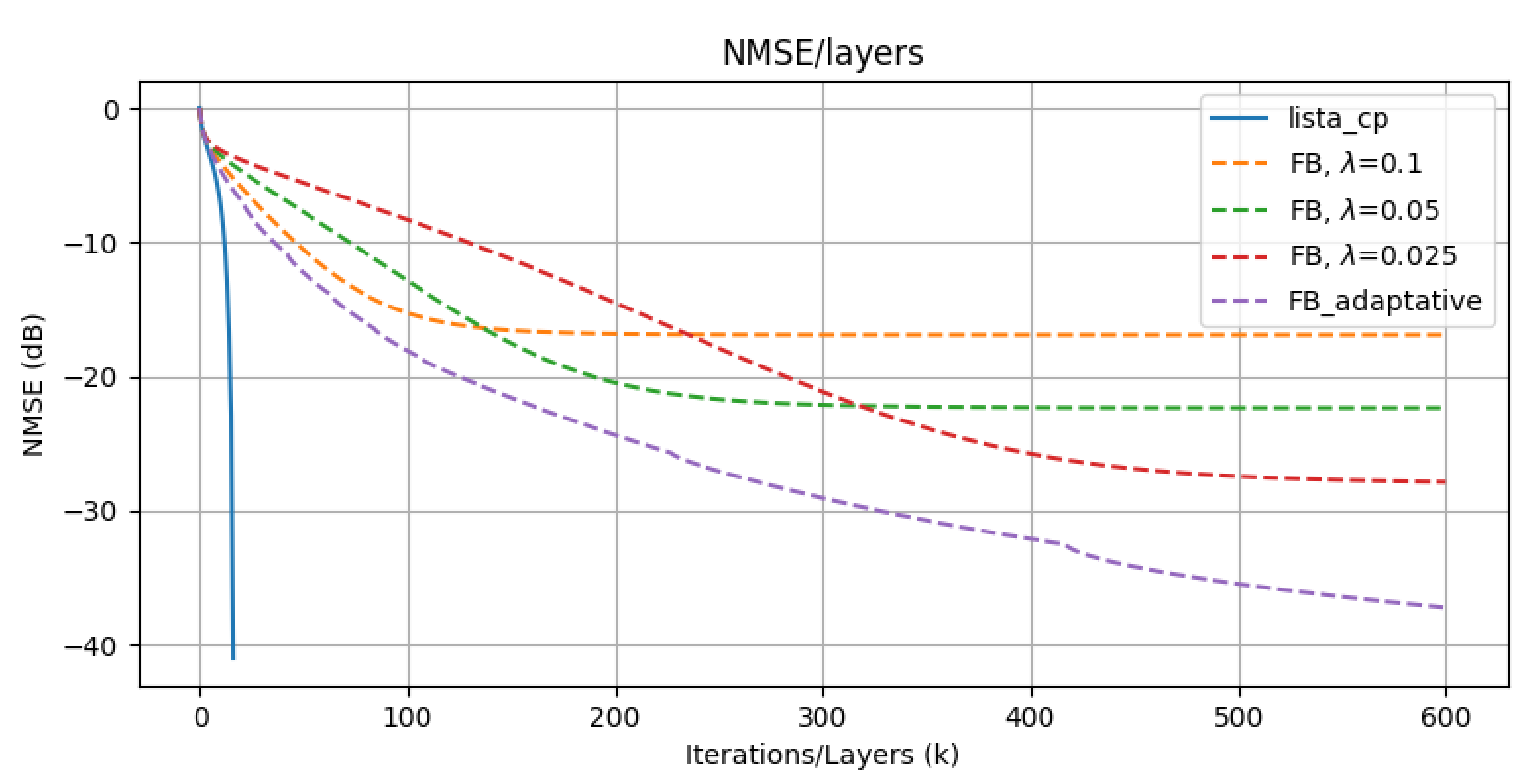

LISTA-SS and LISTA-CPSS

LISTA-SS is a special thresholding scheme, with Support Selection (SS), which is inspired by the article Fast Linearized Bregman Iteration for Compressive Sensing and Sparse Denoising. This technique shows advantages on recoverability and convergence.

The layers of LISTA-SS is defined as LISTA but with a diferent actionvation function:

\[x^{k+1}=\eta_{\mathrm{ss}_{\theta^{k}}}^{p^{k}}\left(W_{2}^{k} x^{k} + W_{1}^{k} y\right), \quad k=0, \cdots, K-1\]

where $\eta_{s s}$ is the thresholding operator with support selection, formally defined as:

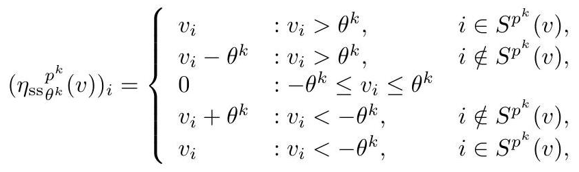
where $S^{p^{k}}(v)$ includes the elements with the largest $p^{k} \%$ magnitudes in vector $v$ :

\[S^{p^{k}}(v)=\left\{i_{1}, i_{2}, \cdots, i_{p^{k}}|| v_{i_{1}}|\geq| v_{i_{2}}|\geq \cdots| v_{i_{p^{k}}}|\cdots \geq| v_{i_{n}} \mid\right\}\]

To summarize, $p^{k}$ is a hyperparameter to be manually tuned, and $\theta^{k}$ is a parameter to train. We use an empirical formula to select $p^{k}$ for layer $k: p^{k}=\min \left( k, 5\right)$.

If we adopt the partial weight coupling we obtain LISTA-CPSS:

\[\begin{align} x^{k+1}=\eta_{\mathrm{ss}} \theta_{\theta^{k}}^{k}\left(\left(\mathbb{I}-W^{k} A\right)x^k + W^{k}y\right), \quad k=0,1, \cdots, K-1 \end{align}\]

This support selection permits to proove a second convergence theorem.

$\textbf{Assumption 2:}$ Signal $x^{*}$ and observation noise $\varepsilon$ are sampled from the following set:

\[\left(x^{*}, \varepsilon\right) \in \overline{\mathcal{X}}(B, \underline{B}, s, \sigma) \triangleq\left\{\left(x^{*}, \varepsilon\right)|| x_{i}^{*} \mid \leq B, \forall i,\left\|x^{*}\right\|_{1} \geq \underline{B},\left\|x^{*}\right\|_{0} \leq s,\|\varepsilon\|_{1} \leq \sigma\right\} .\]

$\textbf{Theorem 3 (LISTA-CPSS):}$ Given $\left\{W^{k}, \theta^{k}\right\}_{k=0}^{\infty}$ and $x^{0}=0$, let $\left\{x^{k}\right\}_{k=1}^{\infty}$ be generated by (6). With the same assumption and parameters as in Theorem 2, the approximation error can be bounded for all $\left(x^{*}, \varepsilon\right) \in \mathcal{X}(B, s, \sigma)$:

\[\begin{align} \left\|d^k_\theta(y)-x^{*}\right\|_{2} \leq s B \exp \left(-\sum_{t=0}^{k-1} c_{\mathrm{ss}}^{t}\right)+C_{\mathrm{ss}} \sigma, \quad \forall k=1,2, \cdots \end{align}\]

where $c_{\mathrm{ss}}^{k} \geq c$ for all $k$ and $C_{\mathrm{ss}} \leq C$.

If Assumption 2 holds, $s$ is small enough, and $\underline{B} \geq 2 C \sigma$ (SNR is not too small), then there exists another sequence of parameters $\left\{\tilde{W}^{k}, \tilde{\theta}^{k}\right\}$ that yields the following improved error bound: for all $\left(x^{*}, \varepsilon\right) \in \overline{\mathcal{X}}(B, \underline{B}, s, \sigma)$,

\[\begin{align} \left\|d^k_\theta(y)-x^{*}\right\|_{2} \leq s B \exp \left(-\sum_{t=0}^{k-1} \tilde{c}_{\mathrm{ss}}^{t}\right)+\tilde{C}_{\mathrm{ss}} \sigma, \quad \forall k=1,2, \cdots \end{align}\]

where $\tilde{c}_{\mathrm{ss}}^{k} \geq c$ for all $k$, $\tilde{c}_{\mathrm{ss}}^{k}>c$ for large enough $k$, and $\tilde{C}_{\mathrm{ss}}<C$.

The bound in (7) ensures that, with the same assumptions and parameters, LISTA-CPSS is at least no worse than LISTA-CP. The bound in (8) shows that, under stronger assumptions, LISTA-CPSS can be strictly better than LISTA-CP in both folds: $\tilde{c}_{\mathrm{ss}}^{k}>c$ is the better convergence rate of LISTA-CPSS; $\tilde{C}_{\mathrm{ss}}<C$ means that the LISTA-CPSS can achieve smaller approximation error than the minimum error that LISTA can achieve. The following results suggests that we can learn parameters of the theorem 2 and 3.LISTA_CP ,LISTA_SS and LISTA_CPSS reach better results than LISTA.