Colour transfert with optimal transport method
Introduction
The objective is to transfer the colormap of an image to make it match that of a target image using optimal transport theory. The code to reproduce the results is available on my GitHub account. The algorithm developed and theory come from the articles Automated colour grading using colour distribution transfer and Wasserstein Barycenter and Its Application to Texture Mixing.
Representation of the images
Because we are interested only in the colors, one image is modeled as a point cloud of \(\mathbb{R}^3\) with a number of points equal to the number of pixels in the image. This means that \(X=\{x_i\}_{i \in [1,N]}\) with \(x_i \in \mathbb{R}^3\) represents an image. If we permute the pixels of an image, it’s representation remains the same. Thus we work in:
\(\mathcal{M}=\{[X]; X \in (\mathbb{R}^3)^N \}\) with \([X]=\{(X_{\sigma(j)})_{j=[1,N]}, \sigma \in \Sigma_N\}\), \(\Sigma_N\) is the set of all permutations.
Wasserstein Distance
We define the Wasserstein distance on \(\mathcal{M}\) :
\(\forall X,Y \in \mathcal{M}, W(X, Y)^{2}={\min\limits_{\sigma \in \Sigma_{N}}} W_{\sigma}(X, Y) \quad \text { where } \quad W_{\sigma}(X, Y)={\sum\limits_{i \in I}}\left\|X_{i}-Y_{\sigma(i)}\right\|^{2}\)
This minimization problem can be computationally expensive, but we can leverage the scalar case (when \(X_i\) and \(Y_i\) are in \(\mathbb{R}\) for \(i \in [1, N]\) instead of being in \((\mathbb{R}^3)^N\)).
In this case \(W(X, Y)=W_{\sigma^*}(X, Y)\) with \(\sigma^*=\sigma_Y \circ \sigma_X^{-1}\) where :
\(\forall 1 \leq i \leq N, \quad X_{\sigma_{X}(i)} \leq X_{\sigma_{X}(i+1)} \quad \text { and } \quad Y_{\sigma_{Y}(i)} \leqslant Y_{\sigma_{Y}(i+1)}\)
It is not computationally costly to calculate \(\sigma\) with fast sorting algorithms.
Then we define the sliced Wasserstein Distance \(\tilde{W}\) which is calculated with only 1-D Wasserstein Distances and approximates the wesserstein Distance as follows:
\(\forall X, Y \in \mathcal{M}, \tilde{W}(X, Y)^{2}=\int_{\theta \in S^2} {\min\limits_{\sigma_{\theta} \in \Sigma_{N}}} {\sum\limits_{i \in I}} \left\langle X_{i}-Y_{\sigma_{\theta}(i)}, \theta\right\rangle^{2} \mathrm{~d} \theta\)
This calculate the Wasserstein Distance using the projected vectors in a certain direction of \(\mathbb{R}^3\) and integrates over all directions. For more details, you can refer to the articles mentioned in the introduction.
Barycenter in Wasserstain Space
Here we define the barycenter in this space and provide an algorithm to obtain the barycenter of the image we want to transport, weighted at 0, and the image with the desired colormap, weighted at 1.
By analogy with the barycenter in Euclidean space, the barycenter in \((\mathcal{M}, \tilde{W})\) is defined as :
\(\operatorname{Bar}\left(\lambda_{j}, Y^{j}\right)_{j \in J} \in \underset{X}{\operatorname{argmin}} E(X)\) where \(E(X)={\sum\limits_{j \in J}}\lambda_{j} \tilde{W}\left(X_\theta, Y_\theta^{j}\right)^{2}=\int_{\theta \in S^2}{\sum\limits_{j \in J}}\lambda_j \left\langle X_{i}-Y_{\sigma^*_{\theta}(i)}, \theta\right\rangle^{2} \mathrm{~d} \theta\)
With \(X_\theta=\{<X_i,\theta>\}_{i\in[1,N]}\subset \mathbb{R}\) and the \(\sigma^*_\theta\) defined in Wasserstein Distance part.
The transportation algorithm:
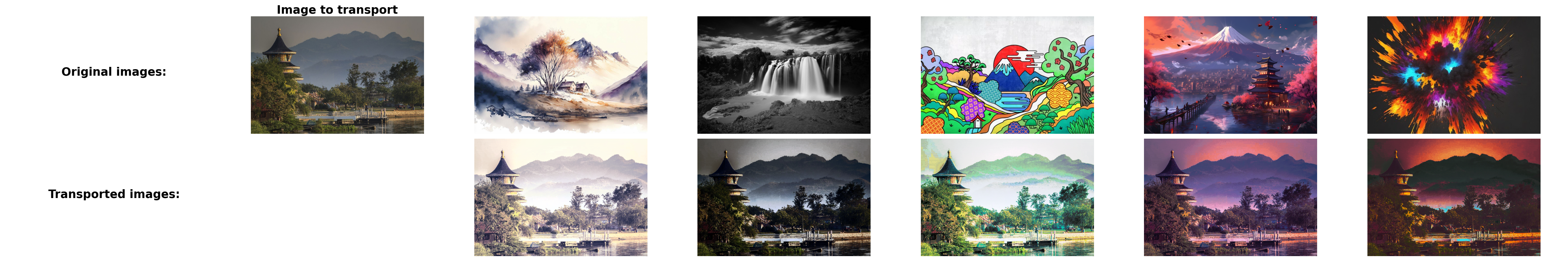
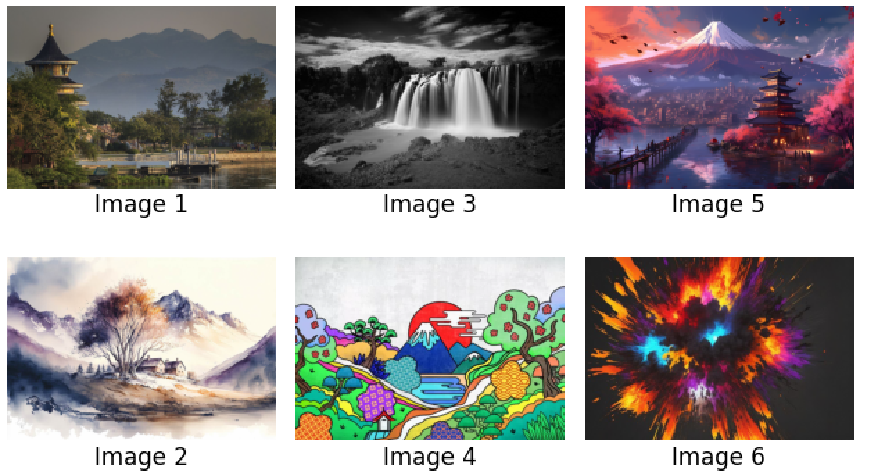
We apply the Wasserstein barycenter with \(\{(0,X);(1,Y)\}\) with \(X\) as the original image (Image 1 in the following figure) we want to transform and \(Y\) as the target image (one of the 5 others) that we want to use to transform \(X\) and use colors.
\(\,\)
Thus the transported image is defined as:
\(\begin{align} X^*=\arg{\min\limits_X}\int_{\theta \in S^2}W(X_\theta, Y_\theta)^2 \mathrm{~d} \theta\end{align}\)
We can use gradient descent to find an approximation of this minimizer:
Gradient descent to minimize (1):
Assumption: Images \(X\) and \(Y\) have the same number of pixels.
Input: \(X\), \(Y\) and a stepsize \(\epsilon\)
\(X^{0}=X\)
For \(k = 0, 1, 2, \ldots\):
\(\quad \quad X^{k}=X^{k}-\epsilon\nabla W(X^{k}_\theta, Y_\theta)\) with \(\theta\) a realization of an uniform random variable in \(S^2\)
Output: \(\lim\limits_{k\rightarrow\infty}{X^k} \in \arg{\min\limits_X}\int_{\theta \in S^2}W(X_\theta, Y_\theta)^2 \mathrm{~d} \theta\)
- Remark: At each step, we pick a direction in the color space and take a step of gradient descent to make the colormap of the current iteration closer to the one of \(Y\) in that direction.
Results
Here are the results obtained by applying the algorithm with 100 iterations and \(\epsilon=1\) to transport the first image, \(X\), to the colormap of the 5 other images, denoted as \(Y\):